Startup-Success-Prediction

import time
from selenium import webdriver
from bs4 import BeautifulSoup
import pandas as pd
import requests
from urllib.request import Request, urlopen
import json
import re
import glob
import os
import numpy as np
import matplotlib as mpl
from matplotlib import pyplot as plt
%matplotlib inline
import warnings
from decimal import Decimal
import math
import seaborn as sns
from scipy.stats import chi2_contingency
from scipy import misc
from matplotlib.colors import ListedColormap
import sklearn
from sklearn import metrics
from sklearn.model_selection import train_test_split
from sklearn import tree
from sklearn.model_selection import GridSearchCV
from sklearn.metrics import make_scorer
from sklearn.ensemble import RandomForestClassifier
from sklearn import linear_model, metrics, preprocessing
from sklearn.preprocessing import StandardScaler, MinMaxScaler
from sklearn.linear_model import LogisticRegression, LinearRegression
from sklearn.metrics import r2_score, f1_score
from sklearn.decomposition import PCA
from sklearn.preprocessing import MinMaxScaler
from sklearn.preprocessing import minmax_scale
from sklearn.neighbors import KNeighborsClassifier
from sklearn.model_selection import cross_val_score
from sklearn.naive_bayes import GaussianNB
from IPython.display import Image, display  
from collections import Counter
import pydotplus 

warnings.filterwarnings("ignore")
pd.set_option('display.max_rows', 500)
pd.set_option('display.max_columns', 500)
pd.set_option('display.width', 1000)

1.1 Scraping - Selenium Infinite Scrolling

html_companies_page = 'https://finder.startupnationcentral.org/startups/search'

def get_driver():
    driver = webdriver.Firefox(executable_path=r'C:\Python34\geckodriver.exe')
    driver.get(html_companies_page)
    return driver

We couldnt get all pages with requests, so we had to use selenium to implement infinite scroll so we can get all companies urls and later on scrape data from this pages.

def infinite_scroll(driver):
    time.sleep(2)  # Allow 2 seconds for the web page to open
    scroll_pause_time = 1 
    screen_height = driver.execute_script("return window.screen.height;")   # get the screen height of the web
    i = 2
    while (i < 50):
        # scroll one screen height each time
        driver.execute_script("window.scrollTo(0, {screen_height}*{i});".format(screen_height=screen_height, i=i))  
        i += 1
        time.sleep(scroll_pause_time)
        scroll_height = driver.execute_script("return document.body.scrollHeight;")  

driver = get_driver()

infinite_scroll(driver)

#linkedin login
driver = get_driver()
username = driver.find_element_by_id('username')
username.send_keys('yair.sultanv@gmail.com')

time.sleep(0.5)

password = driver.find_element_by_id('password')
password.send_keys('yairsultan')

time.sleep(0.5)

log_in_button = driver.find_element_by_class_name('btn__primary--large')
log_in_button.click()

time.sleep(3)

1.2 Scraping - Get Companies Urls

def load_soup_object(html_file_name):
    html = open( html_file_name, encoding="utf8")
    soup = BeautifulSoup(html, 'html.parser')
    return soup

We had to split our requests to multiple files because after some time of infinite scorling we got blocked.

def extract_companies_urls(html_link):
    html_link = "./Data/companies_urls/" + html_link
    soup = load_soup_object(html_link)
    companie_div = soup("div",attrs = {"class" : 'js-company-cards-list'})[0]
    links = list()
    for row in companie_div('div',attrs = {"class" : 'box-view-item'}):
        url = row('a')[0]['href']
        links.append(url)
    return links
      

From each HTML page with multiple companies urls, we extracted the urls in to one big dataframe.

list_50_to_90 = extract_companies_urls('Start-Up1950-1990.html')

list_91_to_00 = extract_companies_urls('Start-Up1991-2000.html')

list_01_to_05 = extract_companies_urls('Start-Up2001-2005.html')

list_05_to_09 = extract_companies_urls('Start-Up2005-2009.html')

list_10_to_11 = extract_companies_urls('Start-Up2010-2011.html')

list_12 = extract_companies_urls('Start-Up2012.html')

list_13 = extract_companies_urls('Start-Up2013.html')

list_14 =extract_companies_urls('Start-Up2014.html')

list_15 = extract_companies_urls('Start-Up2015.html')

list_16 = extract_companies_urls('Start-Up2016.html')

list_17 = extract_companies_urls('Start-Up2017.html')

list_18 = extract_companies_urls('Start-Up2018.html')

list_19 = extract_companies_urls('Start-Up2018.html')

list_20_22 = extract_companies_urls('Start-Up2020-2022.html')

link_list = list_50_to_90 + list_91_to_00 +list_01_to_05+list_05_to_09+ list_10_to_11 + list_12+list_13 + list_14 +list_15 +list_16 +list_17 +list_18 + list_19 +list_20_22  

df = pd.DataFrame({'links' : link_list})

df = df.drop_duplicates().copy()

df = df.reset_index(drop=True)

We ended up with csv file with more then 10,300 urls and saved it.

df.to_csv("companies_urls.csv",index = False)

1.3 Scraping - Company Page Scraping

def load_csv(fileName):
    return pd.read_csv(fileName)

def load_soup_html(url):    
    html = requests.get(url)
    soup = BeautifulSoup(html.text, 'html.parser')
    return soup

Let’s load our urls csv from previous stage :

df = load_csv("companies_urls.csv")

Let’s define a function that extracts all of the features we want from the company page :

def get_df_companies(df):
    res_df = pd.DataFrame(columns=['COMPANIE_NAME', 'FOUNDED', 'BUSINESS_MODEL', 'EMPLOYEES','FUNDING_STAGE','RAISED'
                                   , 'PRODUCT_STAGE', 'NEWS_COUNT', 'FOUNDER_COUNT', 'TOTAL_ROUNDS', 'INVESTORS_COUNT'
                                   , 'COMPANY_STATUS', 'IS_ACADEMIC', 'SECTOR', 'TARGET_INDUSTORY'])
    for url in df['links']:
        print(url)
        soup = load_soup_html(url)
        
        company_dict = {
            "NAME": None,
            "FOUNDED": None,
            "BUSINESS MODEL": None,
            "EMPLOYEES": None,
            "FUNDING STAGE": None,
            "RAISED": 0,
            "PRODUCT STAGE": None,
            "NEWS": 0,
            "FOUNDERS": 0,
            "Total rounds": 0,
            "Investors": 0,
            "STATUS": "Active",
            "IS ACADEMIC": 0,
            "SECTOR": None,
            "TARGET INDUSTORY": None
        }
        
        name_div = soup("div",attrs = {"class" : 'top-profile-section'})
        if(not name_div):
            continue
            
        company_dict["NAME"] = soup("div",attrs = {"class" : 'top-profile-section'})[0]("div",attrs = {"class" : 'title'})[0].get_text().strip()

        COMPANY_PROFILE = soup("div",attrs = {"class" : 'metadata-wrapper'})
        if(len(COMPANY_PROFILE)):
            for div in COMPANY_PROFILE[0]("div",attrs = {"class" : 'item-bottom'}):
                company_dict.update( {div.get_text().strip(): div.find_previous('div').get_text().strip()})
            
        if(soup("div", attrs = {"id": "news-section"})):
            news_div = soup("div", attrs = {"id": "news-section"})[0]
            news_str = news_div("div", attrs = {"class": "section-text"})[0].get_text().strip()
            company_dict["NEWS"] = int(re.findall('\d+', news_str)[0])
            
        if(soup("div", attrs = {"id": "team-section"})):
            team_div = soup("div", attrs = {"id": "team-section"})[0]
            team_str = team_div("div", attrs = {"class": "section-text"})[0].get_text().strip()
            company_dict["FOUNDERS"] = int(re.findall('\d+', team_str)[0])
         
        FUNDING_DATA = soup("div",attrs = {"class" : 'funding-metadata'})
        if(len(FUNDING_DATA)):
            for div in FUNDING_DATA[0]("div",attrs = {"class" : 'subtitle'}):
                funding_text = div.get_text().strip()
                if(funding_text == 'Total rounds' or funding_text == 'Investors'):
                    company_dict[funding_text] = div.find_previous('div').get_text().strip()

        if(soup.find_all("div", string=["Public"])):
            company_dict["STATUS"] = "Public"
        elif(soup.find_all("div", string=["Acquired by"])):
            company_dict["STATUS"] = "Acquired"
        elif(soup.find_all("div", string=["Not Active"])):
            company_dict["STATUS"] = "Not Active"
            
        if(soup.find_all("div", string=["Academic technology"])):
            company_dict["IS ACADEMIC"] = 1
            
        sector_div = soup.find_all("use", attrs={"xlink:href": "#icon-classification-sector"})
        if(sector_div):
            sector_div = sector_div[0].parent.parent.parent.parent("a", attrs = {"class": "lead-title"})
            company_dict["SECTOR"] = sector_div[0].get_text().strip()
        
        industry_div = soup.find_all("use", attrs={"xlink:href": "#icon-classification-industry"})
        if(industry_div):
            industry_div = industry_div[0].parent.parent.parent.parent("a", attrs = {"class": "lead-title"})
            company_dict["TARGET INDUSTORY"] = industry_div[0].get_text().strip()
        
        print(company_dict)
        res_df.loc[len(res_df)] = list(company_dict.values())
        
    return res_df

Main company page with some interesting data!

COMPANY PROFILE data and HTML locators

COMPANY FOUNDERS and Funding rounds timeline

Now, we are going run in a loop, each iteration will include 100 companies data extracting and we will wait a few seconds so we wont get blocked.

Each iteration is saved in a seperate DataFrame so we can be in control all the time and check the data we are getting. (this step lasted about 48 hours)

for i in range(0,104):
    df_res = get_df_companies(df.iloc[i*100: (i+1) * 100])
    df_res.to_csv("Data\companies_df\companies_" + str(i*100) + "-" + str((i*100) + 99) + ".csv",index = False)
    print("************************ file number:" + str(i) + "***********************\n\n")
    time.sleep(10)

Now after we finished scraping all of the data, lets combine all the files to one big DataFrame :

path = r'Data\companies_df'
all_files = sorted(glob.glob(os.path.join(path, "*.csv")), key=os.path.getmtime) #get all files sorted by time modified asc 

df_from_each_file = (pd.read_csv(f) for f in all_files)
concatenated_df = pd.concat(df_from_each_file, ignore_index=True)
# concatenated_df

filepath = r'Data\companies_df\main_df.csv'
concatenated_df.to_csv(filepath, index=False)

2. Data cleaning 🧹🧹🧹

After the scraping process we need to start the cleaning process.

main_df = pd.read_csv('Data/companies_df/main_df.csv')

main_df

	COMPANIE_NAME	FOUNDED	BUSINESS_MODEL	EMPLOYEES	FUNDING_STAGE	RAISED	PRODUCT_STAGE	NEWS_COUNT	FOUNDER_COUNT	TOTAL_ROUNDS	INVESTORS_COUNT	COMPANY_STATUS	IS_ACADEMIC	SECTOR	TARGET_INDUSTORY
0	Golan Plastic Products	1/1964	B2B, B2G	11-50	Public	0	Released	1	4	0	0	Public	0	Industrial Technologies	Energy, Utilities & Waste Management
1	Cham Foods	12/1970	B2B, B2B2C	11-50	Public	0	Released	2	2	0	0	Public	0	AgriFood-tech & Water	Agriculture & Food
2	HerbaMed	1/1986	B2B, B2C	1-10	Revenue Financed	0	Released	2	2	0	0	Not Active	0	AgriFood-tech & Water	Agriculture & Food
3	RAD	1/1981	B2B, B2G	500+	Established	0	Released	13	3	0	0	Active	0	Industrial Technologies	Communication Services
4	RADA	12/1970	B2B, B2G	201-500	Public	$35.3M	Released	31	6	2	5	Public	0	Security Technologies	Defense, Safety & Security
...	...	...	...	...	...	...	...	...	...	...	...	...	...	...	...
10373	Expecting	1/2021	B2B, B2C	11-50	Seed	$1M	Released	2	2	1	0	Active	0	Life Sciences & HealthTech	Consumers
10374	Loona	8/2020	B2B	1-10	Bootstrapped	0	Customer development	0	2	0	0	Active	0	Enterprise, IT & Data Infrastructure	Industrial Manufacturing
10375	Quiz Beez	6/2021	B2C	1-10	Bootstrapped	0	Customer development	0	1	0	0	Active	0	Content & Media	Education
10376	Eureka Security	10/2021	B2B	11-50	Seed	$8M	Released	2	2	1	7	Active	0	Security Technologies	Enterprise & Professional Services
10377	Kitchezz	11/2020	B2B, B2C	1-10	Bootstrapped	0	Released	0	2	0	0	Active	0	Retail & Marketing	Commerce & Retail

10378 rows × 15 columns

First, Let's look at none values for our companies.
We can see that we have up to 709 None values in some columns, so we will start our data cleaning by using dropna.

main_df.isnull().sum(axis = 0)

COMPANIE_NAME         0
FOUNDED             376
BUSINESS_MODEL      467
EMPLOYEES           408
FUNDING_STAGE       709
RAISED                0
PRODUCT_STAGE       569
NEWS_COUNT            0
FOUNDER_COUNT         0
TOTAL_ROUNDS          0
INVESTORS_COUNT       0
COMPANY_STATUS        0
IS_ACADEMIC           0
SECTOR              343
TARGET_INDUSTORY    394
dtype: int64

main_df.dropna(inplace=True)
print(main_df.isnull().sum(axis = 0))
print(len(main_df))

COMPANIE_NAME       0
FOUNDED             0
BUSINESS_MODEL      0
EMPLOYEES           0
FUNDING_STAGE       0
RAISED              0
PRODUCT_STAGE       0
NEWS_COUNT          0
FOUNDER_COUNT       0
TOTAL_ROUNDS        0
INVESTORS_COUNT     0
COMPANY_STATUS      0
IS_ACADEMIC         0
SECTOR              0
TARGET_INDUSTORY    0
dtype: int64
9210

Second, lets see if we can drop duplicate rows.
After removing Nan values we got total of 9210 rows.

main_df.drop_duplicates()

	COMPANIE_NAME	FOUNDED	BUSINESS_MODEL	EMPLOYEES	FUNDING_STAGE	RAISED	PRODUCT_STAGE	NEWS_COUNT	FOUNDER_COUNT	TOTAL_ROUNDS	INVESTORS_COUNT	COMPANY_STATUS	IS_ACADEMIC	SECTOR	TARGET_INDUSTORY
0	Golan Plastic Products	1/1964	B2B, B2G	11-50	Public	0	Released	1	4	0	0	Public	0	Industrial Technologies	Energy, Utilities & Waste Management
1	Cham Foods	12/1970	B2B, B2B2C	11-50	Public	0	Released	2	2	0	0	Public	0	AgriFood-tech & Water	Agriculture & Food
2	HerbaMed	1/1986	B2B, B2C	1-10	Revenue Financed	0	Released	2	2	0	0	Not Active	0	AgriFood-tech & Water	Agriculture & Food
3	RAD	1/1981	B2B, B2G	500+	Established	0	Released	13	3	0	0	Active	0	Industrial Technologies	Communication Services
4	RADA	12/1970	B2B, B2G	201-500	Public	$35.3M	Released	31	6	2	5	Public	0	Security Technologies	Defense, Safety & Security
...	...	...	...	...	...	...	...	...	...	...	...	...	...	...	...
10373	Expecting	1/2021	B2B, B2C	11-50	Seed	$1M	Released	2	2	1	0	Active	0	Life Sciences & HealthTech	Consumers
10374	Loona	8/2020	B2B	1-10	Bootstrapped	0	Customer development	0	2	0	0	Active	0	Enterprise, IT & Data Infrastructure	Industrial Manufacturing
10375	Quiz Beez	6/2021	B2C	1-10	Bootstrapped	0	Customer development	0	1	0	0	Active	0	Content & Media	Education
10376	Eureka Security	10/2021	B2B	11-50	Seed	$8M	Released	2	2	1	7	Active	0	Security Technologies	Enterprise & Professional Services
10377	Kitchezz	11/2020	B2B, B2C	1-10	Bootstrapped	0	Released	0	2	0	0	Active	0	Retail & Marketing	Commerce & Retail

9210 rows × 15 columns

We can see that after drop_duplicates function we still have 9210 rows which means our data scraping done optimally!!!

Now, because our 'RAISED' feature is not numeric, we need to transform our 'RAISED' value from string to int when we take into account the meaning of the letters ('K', 'M', 'B').

d = {'K': 3,'M': 6,'B': 9}
def text_to_num(text):
    if text == '0':return 0
    if text[-1] in d:
        num, magnitude = text[1:-1], text[-1]
        return int(float(num) * 10 ** d[magnitude])
    else:
        return int(0)

for idx, row in main_df.iterrows():
    raised = text_to_num(row['RAISED'])
    main_df.at[idx,'RAISED'] = raised

main_df["RAISED"] = pd.to_numeric(main_df["RAISED"])
main_df["RAISED"].describe().apply(lambda x: format(x, 'f'))

count          9210.000000
mean        9480790.375136
std        49695496.790866
min               0.000000
25%               0.000000
50%               0.000000
75%         1199000.000000
max      1247000000.000000
Name: RAISED, dtype: object

Now, lets extract our month and year from 'FUNDED' feature which looks like this "10/2021".
We need to seperate month and year from each string and push them into our dataframe.

def extract_month_and_year(val):
    lst = val.split('/')
    if len(lst) == 1:
        lst.insert(0,0)
    return int(lst[0]),int(lst[1])

months = list()
years = list()
for idx, row in main_df.iterrows():
    month,year = extract_month_and_year(row['FOUNDED'])
    months.append(month)
    years.append(year)
main_df.insert(loc=2, column='FOUNDED_MONTH', value=months) 
main_df.insert(loc=3, column='FOUNDED_YEAR', value=years) 
main_df.drop(columns = ['FOUNDED'], axis=1, inplace=True)

Let's have a look at our numeric features :

main_df.describe()

	FOUNDED_MONTH	FOUNDED_YEAR	RAISED	NEWS_COUNT	FOUNDER_COUNT	TOTAL_ROUNDS	INVESTORS_COUNT	IS_ACADEMIC
count	9210.000000	9210.000000	9.210000e+03	9210.000000	9210.000000	9210.000000	9210.000000	9210.0
mean	4.998697	2011.541151	9.480790e+06	2.831813	2.618675	0.930293	1.358958	0.0
std	3.775316	9.305594	4.969550e+07	5.668288	1.685656	1.505888	2.841590	0.0
min	0.000000	1950.000000	0.000000e+00	0.000000	0.000000	0.000000	0.000000	0.0
25%	1.000000	2010.000000	0.000000e+00	0.000000	1.250000	0.000000	0.000000	0.0
50%	5.000000	2014.000000	0.000000e+00	1.000000	2.000000	0.000000	0.000000	0.0
75%	8.000000	2017.000000	1.199000e+06	3.000000	3.000000	1.000000	1.000000	0.0
max	12.000000	2022.000000	1.247000e+09	98.000000	41.000000	16.000000	32.000000	0.0

Now we have categorical feature 'BUSINESS_MODEL' that we want to transform to numeric true\false columns :
Buisness model feature has 4 possible categories when there are companies that are characterized by several different models.

def extract_business_model(main_df):
    b2b = list()
    b2c = list()
    b2g = list()
    b2b2c = list()
    for model in main_df['BUSINESS_MODEL']:
        lst = model.split(', ')
        b2b.append('B2B' in lst)
        b2c.append('B2C' in lst)
        b2g.append('B2G' in lst)
        b2b2c.append('B2B2C' in lst)
            
    return b2b, b2c, b2g ,b2b2c
    
    

b2b, b2c, b2g ,b2b2c = extract_business_model(main_df)
main_df.insert(loc=4, column='B2B', value=b2b) 
main_df.insert(loc=5, column='B2C', value=b2c) 
main_df.insert(loc=6, column='B2G', value=b2g) 
main_df.insert(loc=7, column='B2B2C', value=b2b2c) 

main_df['B2B'] = np.where(main_df['B2B'],1,0)
main_df['B2C'] = np.where(main_df['B2C'],1,0)
main_df['B2G'] = np.where(main_df['B2G'],1,0)
main_df['B2B2C'] = np.where(main_df['B2B2C'],1,0)
main_df.drop(columns = ['BUSINESS_MODEL'], axis=1, inplace=True)

'COMPANY_STATUS' is also categorical feature and we want to transform it to numeric true\false columns :

def extract_company_status(main_df):
    is_public = list()
    is_acquired = list()
    is_active = list()
    is_notActive = list()
    for status in main_df['COMPANY_STATUS']:
        is_public.append('Public' == status)
        is_acquired.append('Acquired' == status)
        is_active.append('Active' == status)
        is_notActive.append('Not Active' == status)
    
    is_public = np.where(is_public,1,0)
    is_acquired = np.where(is_acquired,1,0)
    is_active = np.where(is_active,1,0)
    is_notActive = np.where(is_notActive,1,0)
    
    return is_public, is_acquired, is_active ,is_notActive

is_public, is_acquired, is_active ,is_notActive = extract_company_status(main_df)
main_df.insert(loc=16, column='IS_PUBLIC', value=is_public) 
main_df.insert(loc=17, column='IS_ACQUIRED', value=is_acquired) 
main_df.insert(loc=18, column='IS_ACTIVE', value=is_active) 
main_df.insert(loc=19, column='IS_NOT_ACTIVE', value=is_notActive)
main_df.drop(columns = ['COMPANY_STATUS'], axis=1, inplace=True)

Let’s see what we got so far :

main_df

	COMPANIE_NAME	FOUNDED_MONTH	FOUNDED_YEAR	B2B	B2C	B2G	B2B2C	EMPLOYEES	FUNDING_STAGE	RAISED	...	FOUNDER_COUNT	TOTAL_ROUNDS	INVESTORS_COUNT	IS_PUBLIC	IS_ACQUIRED	IS_ACTIVE	IS_NOT_ACTIVE	IS_ACADEMIC	SECTOR	TARGET_INDUSTORY
0	Golan Plastic Products	1	1964	1	0	1	0	11-50	Public	0	...	4	0	0	1	0	0	0	0	Industrial Technologies	Energy, Utilities & Waste Management
1	Cham Foods	12	1970	1	0	0	1	11-50	Public	0	...	2	0	0	1	0	0	0	0	AgriFood-tech & Water	Agriculture & Food
2	HerbaMed	1	1986	1	1	0	0	1-10	Revenue Financed	0	...	2	0	0	0	0	0	1	0	AgriFood-tech & Water	Agriculture & Food
3	RAD	1	1981	1	0	1	0	500+	Established	0	...	3	0	0	0	0	1	0	0	Industrial Technologies	Communication Services
4	RADA	12	1970	1	0	1	0	201-500	Public	35300000	...	6	2	5	1	0	0	0	0	Security Technologies	Defense, Safety & Security
...	...	...	...	...	...	...	...	...	...	...	...	...	...	...	...	...	...	...	...	...	...
10373	Expecting	1	2021	1	1	0	0	11-50	Seed	1000000	...	2	1	0	0	0	1	0	0	Life Sciences & HealthTech	Consumers
10374	Loona	8	2020	1	0	0	0	1-10	Bootstrapped	0	...	2	0	0	0	0	1	0	0	Enterprise, IT & Data Infrastructure	Industrial Manufacturing
10375	Quiz Beez	6	2021	0	1	0	0	1-10	Bootstrapped	0	...	1	0	0	0	0	1	0	0	Content & Media	Education
10376	Eureka Security	10	2021	1	0	0	0	11-50	Seed	8000000	...	2	1	7	0	0	1	0	0	Security Technologies	Enterprise & Professional Services
10377	Kitchezz	11	2020	1	1	0	0	1-10	Bootstrapped	0	...	2	0	0	0	0	1	0	0	Retail & Marketing	Commerce & Retail

9210 rows × 22 columns

main_df.describe(include='all')

	COMPANIE_NAME	FOUNDED_MONTH	FOUNDED_YEAR	B2B	B2C	B2G	B2B2C	EMPLOYEES	FUNDING_STAGE	RAISED	...	FOUNDER_COUNT	TOTAL_ROUNDS	INVESTORS_COUNT	IS_PUBLIC	IS_ACQUIRED	IS_ACTIVE	IS_NOT_ACTIVE	IS_ACADEMIC	SECTOR	TARGET_INDUSTORY
count	9210	9210.000000	9210.000000	9210.000000	9210.000000	9210.000000	9210.000000	9210	9210	9.210000e+03	...	9210.000000	9210.000000	9210.000000	9210.000000	9210.000000	9210.000000	9210.000000	9210.0	9210	9210
unique	9199	NaN	NaN	NaN	NaN	NaN	NaN	5	10	NaN	...	NaN	NaN	NaN	NaN	NaN	NaN	NaN	NaN	11	17
top	Amigo	NaN	NaN	NaN	NaN	NaN	NaN	1-10	Bootstrapped	NaN	...	NaN	NaN	NaN	NaN	NaN	NaN	NaN	NaN	Life Sciences & HealthTech	Consumers
freq	2	NaN	NaN	NaN	NaN	NaN	NaN	5694	2655	NaN	...	NaN	NaN	NaN	NaN	NaN	NaN	NaN	NaN	1660	2640
mean	NaN	4.998697	2011.541151	0.790662	0.338436	0.154397	0.145168	NaN	NaN	9.480790e+06	...	2.618675	0.930293	1.358958	0.035722	0.095331	0.585125	0.283822	0.0	NaN	NaN
std	NaN	3.775316	9.305594	0.406858	0.473203	0.361349	0.352290	NaN	NaN	4.969550e+07	...	1.685656	1.505888	2.841590	0.185606	0.293688	0.492727	0.450876	0.0	NaN	NaN
min	NaN	0.000000	1950.000000	0.000000	0.000000	0.000000	0.000000	NaN	NaN	0.000000e+00	...	0.000000	0.000000	0.000000	0.000000	0.000000	0.000000	0.000000	0.0	NaN	NaN
25%	NaN	1.000000	2010.000000	1.000000	0.000000	0.000000	0.000000	NaN	NaN	0.000000e+00	...	1.250000	0.000000	0.000000	0.000000	0.000000	0.000000	0.000000	0.0	NaN	NaN
50%	NaN	5.000000	2014.000000	1.000000	0.000000	0.000000	0.000000	NaN	NaN	0.000000e+00	...	2.000000	0.000000	0.000000	0.000000	0.000000	1.000000	0.000000	0.0	NaN	NaN
75%	NaN	8.000000	2017.000000	1.000000	1.000000	0.000000	0.000000	NaN	NaN	1.199000e+06	...	3.000000	1.000000	1.000000	0.000000	0.000000	1.000000	1.000000	0.0	NaN	NaN
max	NaN	12.000000	2022.000000	1.000000	1.000000	1.000000	1.000000	NaN	NaN	1.247000e+09	...	41.000000	16.000000	32.000000	1.000000	1.000000	1.000000	1.000000	0.0	NaN	NaN

11 rows × 22 columns

We realized that 'IS_ACADEMIC' value is 0 for all the rows at this point, so we decided to drop the entire column.

print("Number of companies with IS_ACADEMIC = True :  ",sum(main_df['IS_ACADEMIC']==1))
main_df.drop(columns = ['IS_ACADEMIC'], axis=1, inplace=True)

Number of companies with IS_ACADEMIC = True :   0

'FUNDING_STAGE', 'EMPLOYEES' and 'PRODUCT_STAGE' are categorical features and we want to convert their values to numeric categories
Let's look at our unique values :

print(main_df['FUNDING_STAGE'].unique())
print(main_df['EMPLOYEES'].unique())
print(main_df['PRODUCT_STAGE'].unique())

['Public' 'Revenue Financed' 'Established' 'ROUND A' 'ROUND C+' 'Acquired'
 'Seed' 'ROUND B' 'Bootstrapped' 'Pre-Seed']
['11-50' '1-10' '500+' '201-500' '51-200']
['Released' 'Clinical Trial' 'R&D' 'Beta' 'Alpha' 'Customer development']

Acuired is not a funding stage, therefore we need to drop 8 records where funding stage = acuired

len(main_df[main_df['FUNDING_STAGE'] == 'Acquired'].index)

main_df.drop(main_df[main_df.FUNDING_STAGE == 'Acquired'].index, inplace=True)

Because these features are ordinal categorical we want to order them by numerical order :

employees_replace_map = {'1-10': 0, '11-50': 1, '51-200': 2, '201-500': 3, '500+': 4}
main_df['EMPLOYEES'].replace(employees_replace_map, inplace=True)

funding_replace_map = {'Bootstrapped': 0, 'Pre-Seed': 1, 'Seed': 2, 'ROUND A': 3, 'ROUND B': 4, 'ROUND C+': 5, 'Public': 6, 'Revenue Financed': 7, 'Established': 8}
main_df['FUNDING_STAGE'].replace(funding_replace_map, inplace=True)

stage_replace_map = {'Customer development': 0, 'R&D': 1, 'Clinical Trial': 2, 'Alpha': 3, 'Beta': 4, 'Released': 5}
main_df['PRODUCT_STAGE'].replace(stage_replace_map, inplace=True)

'SECTOR' and 'TARGET_INDUSTORY' are not ordinal categorical so we can give them codes in any order.

sector_replace_map = dict( enumerate(main_df['SECTOR'].astype('category').cat.categories ))
main_df['SECTOR'].replace(sector_replace_map, inplace=True)
print(sector_replace_map)
target_replace_map = dict( enumerate(main_df['TARGET_INDUSTORY'].astype('category').cat.categories ))
main_df['TARGET_INDUSTORY'].replace(target_replace_map, inplace=True)
print(target_replace_map)

{0: 'Aerospace & Aviation', 1: 'AgriFood-tech & Water', 2: 'Content & Media', 3: 'Energy-tech', 4: 'Enterprise, IT & Data Infrastructure', 5: 'FinTech', 6: 'Industrial Technologies', 7: 'Life Sciences & HealthTech', 8: 'Retail & Marketing', 9: 'Security Technologies', 10: 'Smart Mobility'}
{0: 'Agriculture & Food', 1: 'Commerce & Retail', 2: 'Communication Services', 3: 'Consumers', 4: 'Defense, Safety & Security', 5: 'Education', 6: 'Energy, Utilities & Waste Management', 7: 'Enterprise & Professional Services', 8: 'Financial Services', 9: 'Food Retail & Consumption', 10: 'Government & City', 11: 'Healthcare & Life Sciences', 12: 'Industrial Manufacturing', 13: 'Media & Entertainment', 14: 'Real Estate & Construction', 15: 'Transportation & Logistics', 16: 'Travel & Tourism'}

def get_age(year_list, month_list):
    age = list()
    for year, month in zip(year_list, month_list):
        age.append((2022 - year) * 365 + (6 - month) * 30)
    return age

We see that we have some months with 0 value so we will replace them with the mean value.

main_df.loc[main_df['FOUNDED_MONTH'] == 0, ['FOUNDED_MONTH']] = round(main_df['FOUNDED_MONTH'].mean())

And now lets add 'AGE' feature which means how old the company is in days.

age = get_age(main_df['FOUNDED_YEAR'], main_df['FOUNDED_MONTH'])
main_df.insert(loc=3, column='AGE', value=age) 

main_df

	COMPANIE_NAME	FOUNDED_MONTH	FOUNDED_YEAR	AGE	B2B	B2C	B2G	B2B2C	EMPLOYEES	FUNDING_STAGE	...	NEWS_COUNT	FOUNDER_COUNT	TOTAL_ROUNDS	INVESTORS_COUNT	IS_PUBLIC	IS_ACQUIRED	IS_ACTIVE	IS_NOT_ACTIVE	SECTOR	TARGET_INDUSTORY
0	Golan Plastic Products	1	1964	21320	1	0	1	0	1	6	...	1	4	0	0	1	0	0	0	Industrial Technologies	Energy, Utilities & Waste Management
1	Cham Foods	12	1970	18800	1	0	0	1	1	6	...	2	2	0	0	1	0	0	0	AgriFood-tech & Water	Agriculture & Food
2	HerbaMed	1	1986	13290	1	1	0	0	0	7	...	2	2	0	0	0	0	0	1	AgriFood-tech & Water	Agriculture & Food
3	RAD	1	1981	15115	1	0	1	0	4	8	...	13	3	0	0	0	0	1	0	Industrial Technologies	Communication Services
4	RADA	12	1970	18800	1	0	1	0	3	6	...	31	6	2	5	1	0	0	0	Security Technologies	Defense, Safety & Security
...	...	...	...	...	...	...	...	...	...	...	...	...	...	...	...	...	...	...	...	...	...
10373	Expecting	1	2021	515	1	1	0	0	1	2	...	2	2	1	0	0	0	1	0	Life Sciences & HealthTech	Consumers
10374	Loona	8	2020	670	1	0	0	0	0	0	...	0	2	0	0	0	0	1	0	Enterprise, IT & Data Infrastructure	Industrial Manufacturing
10375	Quiz Beez	6	2021	365	0	1	0	0	0	0	...	0	1	0	0	0	0	1	0	Content & Media	Education
10376	Eureka Security	10	2021	245	1	0	0	0	1	2	...	2	2	1	7	0	0	1	0	Security Technologies	Enterprise & Professional Services
10377	Kitchezz	11	2020	580	1	1	0	0	0	0	...	0	2	0	0	0	0	1	0	Retail & Marketing	Commerce & Retail

9202 rows × 22 columns

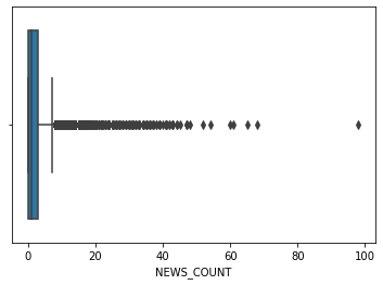
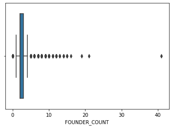
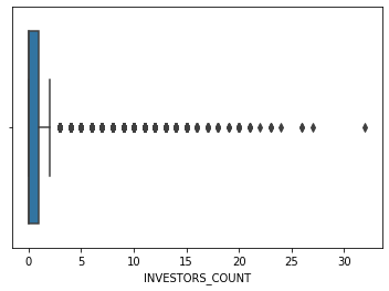
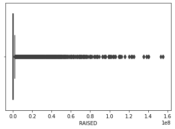
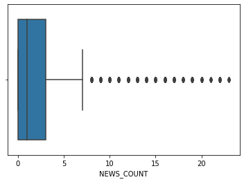
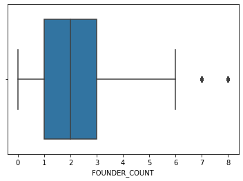
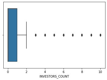
3. Outliers 🤥⛔

In this secion, we are going to:

Detect Outliers and present them by using boxplots for the next features:
- RAISED
- NEWS_COUNT
- FOUNDER_COUNT
- INVESTORS_COUNT
We are going to use Z-score and IQR and select what seems best for us.

sns.boxplot(main_df.RAISED)
plt.show()
sns.boxplot(main_df.NEWS_COUNT)
plt.show()
sns.boxplot(main_df.FOUNDER_COUNT)
plt.show()
sns.boxplot(main_df.INVESTORS_COUNT)
plt.show()

png

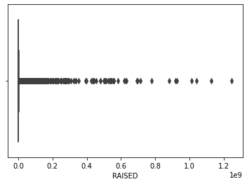
‘RAISED’

Q1 = np.percentile(main_df["RAISED"], 25)
Q3 = np.percentile(main_df["RAISED"], 75)
IQR = Q3 - Q1
print(f"IQR value: {IQR}\nQ1 value: {Q1}\nQ3 value: {Q3}")
Fare_outlier_rows = main_df[(main_df["RAISED"] < Q1 - 1.5*IQR) | (main_df["RAISED"] > Q3 + 1.5*IQR )].index
print("Total sum of outliers detected: ",len(Fare_outlier_rows))

IQR value: 1200000.0
Q1 value: 0.0
Q3 value: 1200000.0
Total sum of outliers detected:  1763

With IQR we got 1763 outliers which is too many, lets try z-score:

z_score = (main_df["RAISED"] - main_df["RAISED"].mean()) / main_df["RAISED"].std()
outliers = abs(z_score) > 3
print("Total outliers: ", sum(outliers))
main_df.drop(main_df[outliers].index, axis=0, inplace=True)
print("110 outliers are much better for us so we will use z-score")

Total outliers:  110
110 outliers are much better for us so we will use z-score

‘NEWS_COUNT’

z_score = (main_df["NEWS_COUNT"] - main_df["NEWS_COUNT"].mean()) / main_df["NEWS_COUNT"].std()
outliers = abs(z_score) > 4
print("Total outliers: ", sum(outliers))
main_df.drop(main_df[outliers].index, axis=0, inplace=True)

Total outliers:  111

‘FOUNDER_COUNT’

z_score = (main_df["FOUNDER_COUNT"] - main_df["FOUNDER_COUNT"].mean()) / main_df["FOUNDER_COUNT"].std()
outliers = abs(z_score) > 4
print("Total outliers: ", sum(outliers))
main_df.drop(main_df[outliers].index, axis=0, inplace=True)

Total outliers:  54

‘INVESTORS_COUNT’

z_score = (main_df["INVESTORS_COUNT"] - main_df["INVESTORS_COUNT"].mean()) / main_df["INVESTORS_COUNT"].std()
outliers = abs(z_score) > 4
print("Total outliers: ", sum(outliers))
main_df.drop(main_df[outliers].index, axis=0, inplace=True)

Total outliers:  106

Let’s look at our features after cleaning outliers:

sns.boxplot(main_df.RAISED)
plt.show()
sns.boxplot(main_df.NEWS_COUNT)
plt.show()
sns.boxplot(main_df.FOUNDER_COUNT)
plt.show()
sns.boxplot(main_df.INVESTORS_COUNT)
plt.show()

png

We can see that our outliers graph for numeric columns are much better now!
Data cleaning is finished, le'ts fix our indexes and save the final data frame.

main_df.reset_index(inplace=True)
main_df

	index	COMPANIE_NAME	FOUNDED_MONTH	FOUNDED_YEAR	AGE	B2B	B2C	B2G	B2B2C	EMPLOYEES	...	NEWS_COUNT	FOUNDER_COUNT	TOTAL_ROUNDS	INVESTORS_COUNT	IS_PUBLIC	IS_ACQUIRED	IS_ACTIVE	IS_NOT_ACTIVE	SECTOR	TARGET_INDUSTORY
0	0	Golan Plastic Products	1	1964	21320	1	0	1	0	1	...	1	4	0	0	1	0	0	0	Industrial Technologies	Energy, Utilities & Waste Management
1	1	Cham Foods	12	1970	18800	1	0	0	1	1	...	2	2	0	0	1	0	0	0	AgriFood-tech & Water	Agriculture & Food
2	2	HerbaMed	1	1986	13290	1	1	0	0	0	...	2	2	0	0	0	0	0	1	AgriFood-tech & Water	Agriculture & Food
3	3	RAD	1	1981	15115	1	0	1	0	4	...	13	3	0	0	0	0	1	0	Industrial Technologies	Communication Services
4	5	Ham-Let	5	1950	26310	1	0	0	0	3	...	7	4	0	0	0	1	0	0	Industrial Technologies	Energy, Utilities & Waste Management
...	...	...	...	...	...	...	...	...	...	...	...	...	...	...	...	...	...	...	...	...	...
8816	10373	Expecting	1	2021	515	1	1	0	0	1	...	2	2	1	0	0	0	1	0	Life Sciences & HealthTech	Consumers
8817	10374	Loona	8	2020	670	1	0	0	0	0	...	0	2	0	0	0	0	1	0	Enterprise, IT & Data Infrastructure	Industrial Manufacturing
8818	10375	Quiz Beez	6	2021	365	0	1	0	0	0	...	0	1	0	0	0	0	1	0	Content & Media	Education
8819	10376	Eureka Security	10	2021	245	1	0	0	0	1	...	2	2	1	7	0	0	1	0	Security Technologies	Enterprise & Professional Services
8820	10377	Kitchezz	11	2020	580	1	1	0	0	0	...	0	2	0	0	0	0	1	0	Retail & Marketing	Commerce & Retail

8821 rows × 23 columns

main_df.to_csv('Data/companies_df/clean_df.csv', index=False)

4. EDA 📊📈📉

df = pd.read_csv('Data/companies_df/clean_df.csv')

df_raised_money = df[df['RAISED'] > 0]
df_didnt_raised_money = df[df['RAISED'] == 0]
print("Total number of companies after cleaning the data: ", len(df))
print("Number of companies who raised money: ",len(df_raised_money))
print("Number of companies who raised money: ",len(df_didnt_raised_money))

Total number of companies after cleaning the data:  8821
Number of companies who raised money:  2905
Number of companies who raised money:  5916

Let’s look at the Status distribution of companies with RAISED money value

fig, axs = plt.subplots(1,3)
fig.subplots_adjust(0.3,0,3,2)

labels = ['IS_PUBLIC', 'IS_ACTIVE', 'IS_ACQUIRED', 'IS_NOT_ACTIVE']

sizes = [len(df[df['IS_PUBLIC'] == 1]), len(df[df['IS_ACTIVE'] == 1]),len(df[df['IS_ACQUIRED'] == 1]), len(df[df['IS_NOT_ACTIVE'] == 1])]
axs[0].pie(sizes, labels=labels,autopct='%1.1f%%',  shadow=True)
axs[0].set_title("All companies", bbox={'facecolor':'0.8', 'pad':5})

sizes_raised = [len(df_raised_money[df_raised_money['IS_PUBLIC'] == 1]), len(df_raised_money[df_raised_money['IS_ACTIVE'] == 1]),len(df_raised_money[df_raised_money['IS_ACQUIRED'] == 1]), len(df_raised_money[df_raised_money['IS_NOT_ACTIVE'] == 1])]
axs[1].pie(sizes_raised, labels=labels,autopct='%1.1f%%',  shadow=True)
axs[1].set_title("Companies with Raised value", bbox={'facecolor':'0.8', 'pad':5})

sizes_didnt_raised = [len(df_didnt_raised_money[df_didnt_raised_money['IS_PUBLIC'] == 1]), len(df_didnt_raised_money[df_didnt_raised_money['IS_ACTIVE'] == 1]),len(df_didnt_raised_money[df_didnt_raised_money['IS_ACQUIRED'] == 1]), len(df_didnt_raised_money[df_didnt_raised_money['IS_NOT_ACTIVE'] == 1])]
axs[2].pie(sizes_didnt_raised, labels=labels,autopct='%1.1f%%',  shadow=True)
axs[2].set_title("Companies without Raised value", bbox={'facecolor':'0.8', 'pad':5})

plt.show()

png

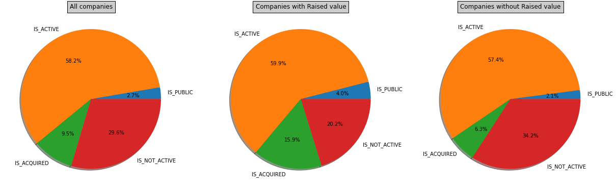
As we can see, companies who raised money are more likely to be aquired or public.

Let’s define what a successful company is:

## - If the company is acquired or public we will consider it a successful company.

df_succeeded_companies = df[(df.IS_ACQUIRED == 1) | (df.IS_PUBLIC == 1)]
df_unsucceeded_companies = df[(df.IS_ACQUIRED == 0) & (df.IS_PUBLIC == 0)]
print("The number of succeeded companies is: ",len(df_succeeded_companies))
print("The number of unSucceeded companies is: ",len(df_unsucceeded_companies))

The number of succeeded companies is:  1073
The number of unSucceeded companies is:  7748

After we defined what a successful company is, we need to convert our 4 status columns to ‘is_successful’ column.

def extract_company_status(main_df):
    is_successful = list()

    for index, row in df.iterrows():
        if(row['IS_PUBLIC'] | row['IS_ACQUIRED']):
            is_successful.append(1)
        else:
            is_successful.append(0)
    
    return is_successful

is_successful = extract_company_status(df)
df.insert(loc=16, column='IS_SUCCESSFUL', value=is_successful)
df.drop(columns = ['IS_PUBLIC'], axis=1, inplace=True)
df.drop(columns = ['IS_ACQUIRED'], axis=1, inplace=True)
df.drop(columns = ['IS_ACTIVE'], axis=1, inplace=True)
df.drop(columns = ['IS_NOT_ACTIVE'], axis=1, inplace=True)
df.drop(columns = ['COMPANIE_NAME'], axis=1, inplace=True)

We will now examine whether the number of employees affects the company’s success.

ct = pd.crosstab(df['EMPLOYEES'], (df['IS_SUCCESSFUL']), normalize="index")

ax = ct.plot(kind="bar", figsize=(18,6), label=["1-10","11-50","51-200","201-500","500+"])
ax.legend(["Unsuccessful", "Successful"],fancybox=True, framealpha=1, shadow=True, borderpad=1)
for container in ax.containers:
    ax.bar_label(container)

plt.title("Number of employees in successful companies", fontsize = 20)
plt.ylabel("Relative frequency")

Text(0, 0.5, 'Relative frequency')

png

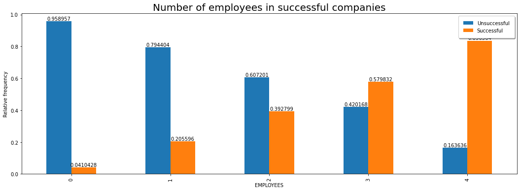
It can certainly be seen that the larger the number of employees, the greater the chances of success.

We tried to check if there is a relationship between the age of a company and the number of company investors

x = df_raised_money.AGE
y = df_raised_money.RAISED
A = np.vstack([x, np.ones(len(x))]).T

y = y[:, np.newaxis]
alpha = np.dot((np.dot(np.linalg.inv(np.dot(A.T,A)),A.T)),y)

plt.figure(figsize = (8,6))
plt.plot(x, y, 'b.')
plt.plot(x, alpha[0]*x + alpha[1], 'r')
plt.xlabel('Age in days')
plt.ylabel('Amount of money raised in Billion $')
plt.show()

png

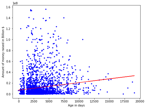
From the graph it can be seen that there is a real connection between the age of the company in days and the amount of money that the company raised. It can be understood from this graph that the longer a company exists, the more likely it is to raise money. And as we have seen before, companies that raise money are more likely to succeed.

We are now trying to test relationships and behaviors between quantitative variables. *

We chose to take the columns:
~EMPLOYEES
~NEWS_COUNT
~FOUNDER_COUNT
~INVESTORS_COUNT

corr = df[['EMPLOYEES', 'NEWS_COUNT', 'FOUNDER_COUNT','INVESTORS_COUNT']].corr()
mask = np.zeros_like(corr)
with sns.axes_style("darkgrid"):
    f, ax = plt.subplots(figsize=(15, 15))
    ax = sns.heatmap(corr, mask=mask, vmax=1, square=True,annot=True)
    
# df = pd.DataFrame(df)
# sns.heatmap(df.corr(), annot=True)

png

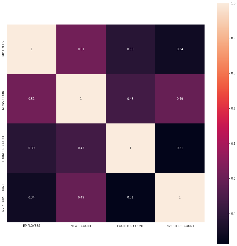
We were able to find out that there is a strong connection between the number of employees in the company and the number of news articles about the company.

ct2 = pd.crosstab(df[(df['RAISED'] == 0)]['TARGET_INDUSTORY'], df[(df['RAISED'] == 0)]['SECTOR'])
ct2

SECTOR	Aerospace & Aviation	AgriFood-tech & Water	Content & Media	Energy-tech	Enterprise, IT & Data Infrastructure	FinTech	Industrial Technologies	Life Sciences & HealthTech	Retail & Marketing	Security Technologies	Smart Mobility
TARGET_INDUSTORY
Agriculture & Food	11	343	1	10	11	3	34	8	1	4	4
Commerce & Retail	1	8	53	10	86	20	44	61	189	19	10
Communication Services	3	0	15	3	24	2	61	2	5	13	5
Consumers	4	32	711	23	169	163	21	293	222	85	87
Defense, Safety & Security	34	0	3	8	16	1	55	11	0	112	8
Education	0	1	33	0	7	1	3	13	0	7	0
Energy, Utilities & Waste Management	2	40	1	65	5	0	40	2	0	17	1
Enterprise & Professional Services	0	2	108	8	552	41	17	10	235	169	5
Financial Services	0	0	1	0	29	80	1	4	5	14	3
Food Retail & Consumption	0	17	5	1	7	0	3	2	15	0	0
Government & City	0	7	2	5	3	1	5	2	1	8	10
Healthcare & Life Sciences	0	12	4	4	12	2	40	608	0	1	0
Industrial Manufacturing	9	8	0	14	12	0	100	1	2	13	23
Media & Entertainment	0	0	126	0	4	1	1	0	24	0	1
Real Estate & Construction	0	4	1	11	9	9	31	0	6	4	0
Transportation & Logistics	2	0	1	0	5	1	6	0	5	3	15
Travel & Tourism	0	0	6	0	12	1	1	1	19	3	0

In this graph we see the distribution of companies by target industory

fig, ax = plt.subplots(figsize=(18, 4))
fg = sns.histplot(df['TARGET_INDUSTORY'], ax=ax)
fg.set_title("Target Industory Histogram")
fg.set_xlabel("Target Industory")
plt.xticks(rotation=90, ha='right', rotation_mode='anchor')
plt.show()

png

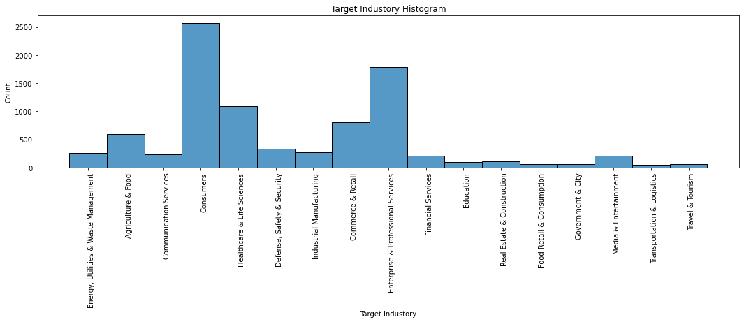
We can seen that the most common sectors are:

Consumers
Enterprise & Professional Services
Life Sciences & HealthTech

We will try to examine information with a large number of columns, to check if the number of companies is divided into several subgroups we will do this using PCA

EDA - Principle Component Analysis (PCA)

Step 1

We create a dataframe containing some numerical variables of our data set:

dataset = df.loc[:,[ 'NEWS_COUNT', 'FOUNDER_COUNT', 'TOTAL_ROUNDS', 'INVESTORS_COUNT','EMPLOYEES','PRODUCT_STAGE']]
dataset.shape

(8821, 6)

Step 2

We now need to create a PCA object, and then call the function that performs PCA on the dataset. the parameter n_componenets, which determines the number of dimesions we would like to have in the end:

pca2 = PCA(n_components=2) #creating a PCA object, while determining the desired number of dimensions
pcComponents = pca2.fit_transform(dataset) #performing PCA using fit_transform on our dataset

PCA creates new axes, hence, new variables - pcComponents is the new numerical data, with two dimensions:

pcComponents.shape

(8821, 2)

Step 3

To make it easy to display our results, we will create a new dataframe with the new features:

principalDf = pd.DataFrame(data = pcComponents, columns = ['principal component 1', 'principal component 2'])
principalDf

	principal component 1	principal component 2
0	-1.057272	-0.672293
1	-0.516033	-1.171117
2	-0.620490	-1.167730
3	9.815548	-5.517506
4	4.519727	-3.071575
...	...	...
8816	-0.311000	-0.760671
8817	-2.873409	-0.201562
8818	-3.050129	-0.251598
8819	1.976308	4.964279
8820	-2.409851	-0.370227

8821 rows × 2 columns

Step 4

We also add the IS_SUCCESSFUL feature, so we will be able to display the data separating successful and unseccessful comapnies:

finalDf = pd.concat([principalDf, df[['IS_SUCCESSFUL']]], axis = 1)

Step 5

We are ready to see our results. We will use a scatterplot:

fig = plt.figure()
ax = plt.axes()
colormap = np.array(['r', 'b'])
ax.scatter(finalDf['principal component 1'], finalDf['principal component 2'], c=colormap[finalDf.IS_SUCCESSFUL])
plt.xlabel('PC1')
plt.ylabel('PC2')
plt.show()

png

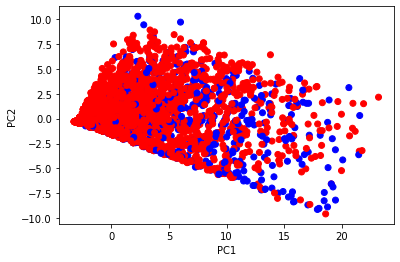
As you can see, we can’t see in this figure a clear separation of successful and unsuccessful companies.

Chi-Square Test of Independence.

We will try to check if there is a relationship between categorical variables.

*EMPLOYEES column
*PRODUCT_STAGE column

ct1 = pd.crosstab(df.PRODUCT_STAGE, df.EMPLOYEES)
ct1

EMPLOYEES	0	1	2	3	4
PRODUCT_STAGE
0	196	8	1	0	0
1	1084	119	2	0	0
2	177	65	3	0	0
3	286	22	1	1	0
4	700	108	3	0	0
5	3234	2037	601	118	55

chi2_contingency(ct1)

(1071.8373864739401,
 1.8320493744078054e-214,
 20,
 array([[1.31933454e+02, 5.48231493e+01, 1.41996372e+01, 2.76555946e+00,
         1.27819975e+00],
        [7.75511280e+02, 3.22253146e+02, 8.34661603e+01, 1.62560934e+01,
         7.51332049e+00],
        [1.57676567e+02, 6.55203492e+01, 1.69702982e+01, 3.30518082e+00,
         1.52760458e+00],
        [1.99509126e+02, 8.29032989e+01, 2.14726222e+01, 4.18206553e+00,
         1.93288743e+00],
        [5.21941617e+02, 2.16885727e+02, 5.61751502e+01, 1.09408230e+01,
         5.05668292e+00],
        [3.89042796e+03, 1.61661433e+03, 4.18716132e+02, 8.15502777e+01,
         3.76913048e+01]]))

We got
- 1071.8373864739401 Chi-Square
- p_vaule < 0.05
We therefore see that there is a relationship between the variables and they are not independent
- PRODUCT_STAGE column
- EMPLOYEES column
From chi square test we have learned that PRODUCT_STAGE and EMPLOYEES features that the higher number of employees is the higher the product stage is and the opposite claim is also true.

df.to_csv('Data/companies_df/eda_df.csv', index=False)

5. Machine Learning 🤖🤖🤖

df = pd.read_csv('Data/companies_df/eda_df.csv')

To start with the machine learning train and prediction, we need to convert our 4 status columns to ‘is_successful’ column.

'SECTOR' and 'TARGET_INDUSTORY' are not ordinal categorical so we can give them codes in any order.

sector_replace_map = dict( enumerate(df['SECTOR'].astype('category').cat.categories ))
sector_replace_map = dict([(value, key) for key, value in sector_replace_map.items()])
df['SECTOR'].replace(sector_replace_map, inplace=True)

target_replace_map = dict( enumerate(df['TARGET_INDUSTORY'].astype('category').cat.categories ))
target_replace_map = dict([(value, key) for key, value in target_replace_map.items()])
df['TARGET_INDUSTORY'].replace(target_replace_map, inplace=True)

We need to predict the ‘IS_SUCCESSFUL’ column. Let us separate it and assign it to a target variable ‘y’. The rest of the data frame will be the set of input variables X.

y = df["IS_SUCCESSFUL"].values
x = df.drop(["IS_SUCCESSFUL"],axis=1)

Now let’s scale the predictor variables and then separate the training and the testing data.

#Divide into training and test data
X_train, X_test, y_train, y_test = train_test_split(x, y, random_state=0 ,test_size = 0.3) # 70% training and 30% test

Logistic Regression

clf = LogisticRegression(solver='lbfgs', max_iter=1000)
clf.fit(X_train, y_train)
y_predict = clf.predict(X_test)
acc = clf.score(X_test,y_test)
print(f"Accuracy of our model using logistic regression: {acc}")

Accuracy of our model using logistic regression: 0.8734416320362675

Lets display our predicted result with confusion matrix

y_predict = clf.predict(X_test)
cf_matrix = metrics.confusion_matrix(y_test, y_predict)

ax= plt.subplot()
sns.heatmap(cf_matrix, annot=True, fmt='g', ax=ax, cmap='Blues');  #annot=True to annotate cells, ftm='g' to disable scientific notation

# labels, title and ticks
ax.set_xlabel('Predicted labels');ax.set_ylabel('True labels'); ax.set_title('Confusion Matrix'); ax.xaxis.set_ticklabels(['False','True']);ax.yaxis.set_ticklabels(['False','True']);

png

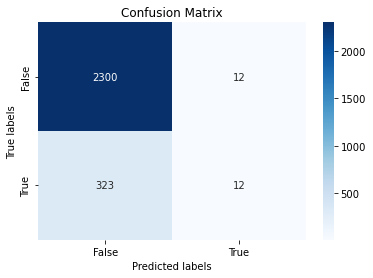
print("accuracy is:",metrics.accuracy_score(y_test, y_predict))
print("precision is:",metrics.precision_score(y_test, y_predict))
print("recall is:",metrics.recall_score(y_test, y_predict))
print("f1 is:",metrics.f1_score(y_test, y_predict))

accuracy is: 0.8734416320362675
precision is: 0.5
recall is: 0.03582089552238806
f1 is: 0.06685236768802229

As we can see the results are not so great, lets try make some changes:

First, We found that ‘TARGET_INDUSTORY’ and ‘FOUNDED_YEAR’ features degrades model performance so we will drop them.

Second, We want to scale our ‘RAISED’ feature because it has very high values.

df.drop(columns = ['TARGET_INDUSTORY'], axis=1, inplace=True)
df.drop(columns = ['FOUNDED_YEAR'], axis=1, inplace=True)

df[['RAISED']] = minmax_scale(df[['RAISED']])


y = df["IS_SUCCESSFUL"].values
x = df.drop(["IS_SUCCESSFUL"],axis=1)

X_train, X_test, y_train, y_test = train_test_split(x, y, random_state=0 ,test_size = 0.3) # 70% training and 30% test

clf = LogisticRegression(solver='lbfgs', max_iter=1000)
clf.fit(X_train, y_train)
y_predict = clf.predict(X_test)

ax= plt.subplot()
cf_matrix = metrics.confusion_matrix(y_test, y_predict)
sns.heatmap(cf_matrix, annot=True, fmt='g', ax=ax, cmap='Blues');  #annot=True to annotate cells, ftm='g' to disable scientific notation
# labels, title and ticks
ax.set_xlabel('Predicted labels');ax.set_ylabel('True labels'); ax.set_title('Confusion Matrix'); ax.xaxis.set_ticklabels(['False','True']);ax.yaxis.set_ticklabels(['False','True']);

png

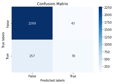
Now lets look at the results again.

print("accuracy is:",metrics.accuracy_score(y_test, y_predict))
print("precision is:",metrics.precision_score(y_test, y_predict))
print("recall is:",metrics.recall_score(y_test, y_predict))
print("f1 is:",metrics.f1_score(y_test, y_predict))

accuracy is: 0.8866641480921799
precision is: 0.6446280991735537
recall is: 0.23283582089552238
f1 is: 0.3421052631578947

As we can see we got about 20-40% higher results!!!

KNN - K-Nearest Neighbors

# set up the model, k-NN classification with k = ?  
k = 3
clf = KNeighborsClassifier(n_neighbors=k)
clf.fit(X_train, y_train)
y_predict = clf.predict(X_test)

cf_matrix = metrics.confusion_matrix(y_true = y_test, y_pred = y_predict)

print('Accuracy = ', metrics.accuracy_score(y_true = y_test, y_pred = y_predict))

Accuracy =  0.8587079712882508

Let us take a few possible values of k and fit the model on the training data for all those values. We will also compute the training score and testing score for all those values.

train_score = []
test_score = []
k_vals = []

for k in range(1, 75):
    k_vals.append(k)
    knn = KNeighborsClassifier(n_neighbors = k)
    knn.fit(X_train, y_train)
    
    tr_score = knn.score(X_train, y_train)
    train_score.append(tr_score)
    
    te_score = knn.score(X_test, y_test)
    test_score.append(te_score)

print(f"Max train_score is: {max(train_score)}\nMax test_score is: {max(test_score)}")

Max train_score is: 1.0
Max test_score is: 0.8745749905553457

plt.figure(figsize=(10,5))
plt.xlabel('Different Values of K')
plt.ylabel('Model score')
plt.plot(k_vals, train_score, color = 'r', label = "training score")
plt.plot(k_vals, test_score, color = 'b', label = 'test score')
plt.legend(bbox_to_anchor=(1, 1),
           bbox_transform=plt.gcf().transFigure)
plt.show()

png

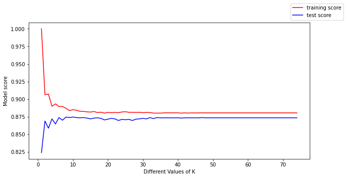
We found the best K for our model!
K = 10
Accuracy = 0.8745749905553457

knn = KNeighborsClassifier(n_neighbors = 10)

#Fit the model
knn.fit(X_train,y_train)

#get the score
knn.score(X_test,y_test)

0.8745749905553457

We can make the following conclusions from the above plot:

For low values of k, the training score is high, while the testing score is low.
As the value of k increases, the testing score starts to increase and the training score starts to decrease.
However, the higher the value of k, both the training score and the testing score are close to each other.

Decision Trees

def splitData(df, features, labels, specifed_random_state=0):
    """Split a subset of the dataset, given by the features, into train and test sets."""
    df_predictors = df[features].values
    df_labels = df[labels].values

    # Split into training and test sets
    XTrain, XTest, yTrain, yTest = train_test_split(df_predictors, df_labels, random_state=specifed_random_state)
    return XTrain, XTest, yTrain, yTest

def renderTree(my_tree, features):
    # hacky solution of writing to files and reading again
    # necessary due to library bugs
    filename = "temp.dot"
    with open(filename, 'w') as f:
        f = tree.export_graphviz(my_tree, 
                                 out_file=f, 
                                 feature_names=features, 
                                 class_names=["Perished", "Survived"],  
                                 filled=True, 
                                 rounded=True,
                                 special_characters=True)
  
    dot_data = ""
    with open(filename, 'r') as f:
        dot_data = f.read()

    graph = pydotplus.graph_from_dot_data(dot_data)
    image_name = "temp.png"
    graph.write_png(image_name)  
    display(Image(filename=image_name))

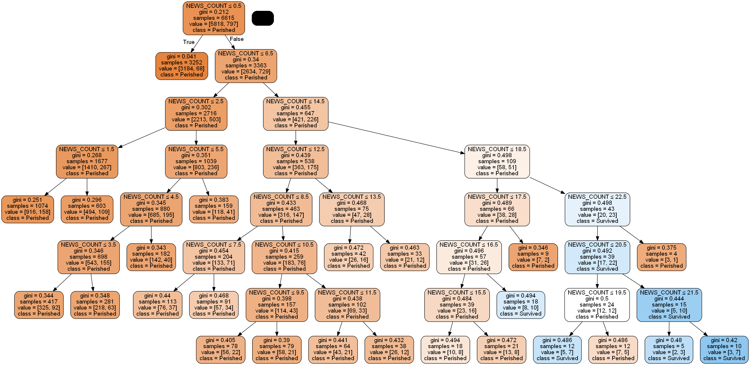
And here you can see the decision tree model with the prediction and accuracy of the training and testing of the model based on ‘NEWS_COUNT’ feature only.

decisionTree = tree.DecisionTreeClassifier()
features = ['NEWS_COUNT']

XTrain, XTest, yTrain, yTest = splitData(df, features, ["IS_SUCCESSFUL"])
# fit the tree with the traing data
decisionTree = decisionTree.fit(XTrain, yTrain)

# predict with the training data
y_pred_train = decisionTree.predict(XTrain)
# measure accuracy
print('Accuracy on training data = ', 
      metrics.accuracy_score(y_true = yTrain, y_pred = y_pred_train))

# predict with the test data
y_pred = decisionTree.predict(XTest)
# measure accuracy
print('Accuracy on test data = ', 
      metrics.accuracy_score(y_true = yTest, y_pred = y_pred))

renderTree(decisionTree, features)

Accuracy on training data =  0.8808767951625095
Accuracy on test data =  0.8739800543970988

png

decisionTree = tree.DecisionTreeClassifier()
all_features = df.columns.tolist()

all_features.remove('IS_SUCCESSFUL')

# fit the tree with the traing data
decisionTree = decisionTree.fit(X_train,y_train)

# predict with the training data
y_predict_train = decisionTree.predict(X_train)
# measure accuracy
print('Accuracy on training data = ', 
      metrics.accuracy_score(y_true = y_train, y_pred = y_predict_train))

# predict with the test data
y_predict = decisionTree.predict(X_test)
# measure accuracy
print('Accuracy on test data = ', 
      metrics.accuracy_score(y_true = y_test, y_pred = y_predict))

renderTree(decisionTree,all_features)

Accuracy on training data =  1.0
Accuracy on test data =  0.8617302606724594
dot: graph is too large for cairo-renderer bitmaps. Scaling by 0.899402 to fit

png

OK, clearly, we’re overfitting the data - 100% accuracy on the training data and only ~86% on the test data. Yet, we’ve created a complicated tree.

decisionTree = tree.DecisionTreeClassifier(max_depth=5, min_samples_split=20)
XTrain, XTest, yTrain, yTest = splitData(df, all_features, ["IS_SUCCESSFUL"])
decisionTree = decisionTree.fit(XTrain, yTrain)

y_pred_train = decisionTree.predict(XTrain)
print('Accuracy on training data= ', metrics.accuracy_score(y_true = yTrain, y_pred = y_pred_train))

y_pred = decisionTree.predict(XTest)
print('Accuracy on test data= ', metrics.accuracy_score(y_true = yTest, y_pred = y_pred))

renderTree(decisionTree, all_features)

Accuracy on training data=  0.8946334089191232
Accuracy on test data=  0.8907524932003626

png

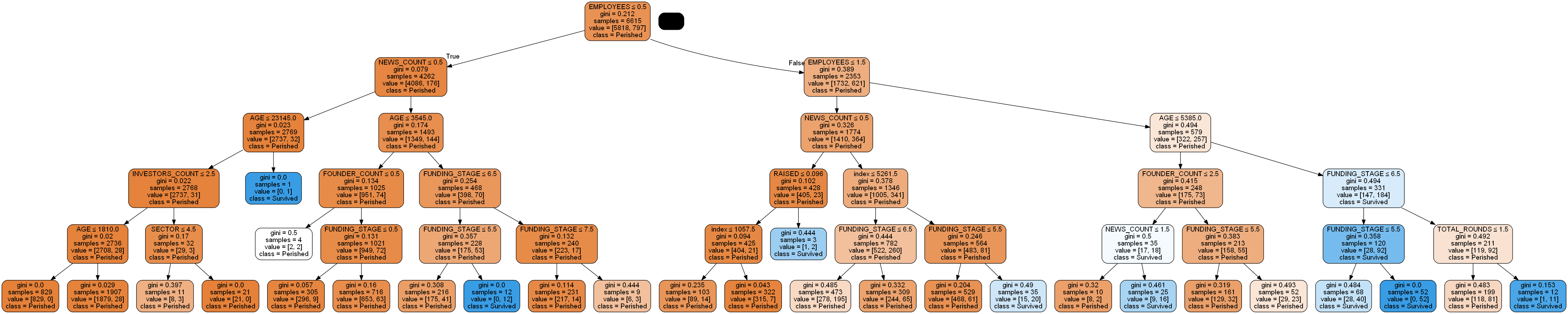
Slight improvement 89% for training and test without overfitting

We got ourselves a better training accuracy but the test prediction did not improve by a noticiable percentage.

Naive Bayes

# Split into training and test sets
y = df["IS_SUCCESSFUL"].values
x = df.drop(["IS_SUCCESSFUL"],axis=1)

XTrain, XTest, yTrain, yTest = train_test_split(x, y, random_state=0, test_size=0.25)

# Instantiate the classifier
gnb = GaussianNB()

gnb.fit(XTrain,yTrain)

y_pred = gnb.predict(XTest)
y_pred_train = gnb.predict(XTrain)

# Print results
print('Accuracy on Train data= ', metrics.accuracy_score(y_true = yTrain, y_pred = y_pred_train))
print('Accuracy on test data= ', metrics.accuracy_score(y_true = yTest, y_pred = y_pred))

Accuracy on Train data=  0.816780045351474
Accuracy on test data=  0.8250226654578422

gnb.class_prior_

array([0.87951625, 0.12048375])

We can see that only about 12% SUCCESSFUL..

In conclusion, we have seen that the algorithms that have brought us the best results are Decision Trees and Logistic Regression with about 89% accuracy.

Credit: part of the code was taken from Data Science course Campus IL

df.to_csv('Data/companies_df/final_df.csv', index=False)